Draw Circle Save Points Along Edge Matlab
voronoi_diagram
voronoi_diagram, but a sketch of some tools that are available for computing the Voronoi diagram of a set of points in the plane. Here, nosotros are more often than not concerned with ways of making pictures of such diagrams, or of determining the location of the vertices of the polygon around each generator.
DIAMOND: A sample dataset
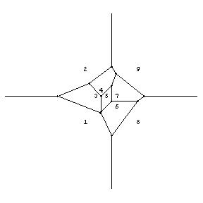
To keep things simple, we'll but be concerned with 2D Voronoi diagrams, and nosotros'll concentrate on a unmarried modest dataset of points whose coordinates are independent in the unit square. Hither is a typewriter plot of the data:
2 . . . . . . . . . 9 . . . . . . . . . . . . . . . . . . . . . . . . . . . . . . . . . . . . 4 . . . . . . . . . 3 . five . vii . . . . . . . . . . . . . . . . . . . . . 6 . . . . . . . . . . . . . . . . . . . . . . . . . . ane . . . . . . . . . eight
Hither are the coordinates of the points:
0.0 0.0 0.0 1.0 0.2 0.five 0.3 0.6 0.4 0.5 0.6 0.3 0.six 0.v 1.0 0.0 1.0 i.0
One useful affair about this dataset is that I can tell yous EXACTLY the shape of the Voronoi polygon around the point labeled 5. Information technology consists of the four points (0.3,0.2), (0.five,0.iv), (0.5,0.seven), and (0.3,0.5), which grade a sort of diamond around the point. This fact should assistance afterward, when we are trying to empathise the output of some of the programs.
What Data Practice We Want?
In some cases, all nosotros want to do is see a flick of the Voronoi diagram. Nosotros will see that at that place are a number of ways of doing that; withal, fifty-fifty for this relatively simply task, in that location are some complications. Some plots don't evidence the rays to infinity. Some are line plots and some fill each region with color.
Often, we want to compute something based on the Voronoi diagram. Permit'southward concentrate on one particular computation, determining the centroid of a Voronoi cell in 2D. To practise this, nosotros need to know the number of vertices in the cell and their locations. We as well need to know their adjacency, that is, the order in which the vertices are placed around the generator.
We'll suppose that nosotros starting time with g_num points in 2D, which we call generators. We have the coordinates of these points, available either equally ii lists g_x(i:g_num), g_y(1:g_num), or as a doubly-dimensioned array g_xy(one:2,ane:g_num). We now suppose that our ideal program has computed the Voronoi diagram, and that it is willing to written report this information using whatever data structure suits u.s.a..
The get-go piece of information we want is v_num, the full number of Voronoi vertices. Next, we want v_xy(1:2,i:v_num), the coordinates of the Voronoi vertices. Next, we want a vector g_degree(one:g_num) that contains the number of Voronoi vertices associated with each jail cell.
So far, information technology's been piece of cake to call back nigh the information and how to shop it, but what about the lists of vertices? We'll want to be able to specify a generator I. From that, we know how to get the number of vertices, g_degree(i). Now let's suppose in that location'south some large array g_face containing the lists, and that the list for generator I starts at g_start(i). Then we'll know that we have to read a full of g_degree(i) successive values to go around the polygon.
Just how practice we handle infinite polygons? These occur any time a generator Yard is part of the convex hull of the point set up. In that case, the Voronoi region is a "polygon" with two semi-space sides. Peradventure the best way to handle this is to pretend that the region is substantially a polygon with one missing side. We imagine that there are "nodes at infinity". The degree of whatsoever Voronoi region with semi-space sides volition be increased by two. The list of vertices in g_face will be adjusted past adding one node at infinity to the beginning of the list, and ane at the end. To indicate that these are special nodes, we will shop them with a negative sign in the entries of g_face.
The number of nodes at infinity will be stored every bit i_num. The "directions" associated with these nodes will be stored in i_xy. To be clear about this, if a ray with direction i_xy(i:2,i) emanates from a Voronoi vertex v_xy(ane:2,j), or if, in other words, finite vertex i is connected to the j-th vertex at infinity, so we intend that the respective ray is the set of points
v_xy(i:ii,j) + southward * i_xy(1:2,i)for all nonnegative values s.
Thus, if we run into a generator whose vertex listing is
( -7, xi, eight, 4, -thirteen),we can draw the Voronoi region by starting with a line in the direction stored in i_xy(one:two,seven) that terminates at v_xy(1:2,11), continue to vertices 8 and four, and so depict a line from v_xy(1:ii,4) in the direction i_xy(1:2,13).
If the but affair nosotros're interested in is a picture of the Voronoi diagram, then it'south possible to greatly simplify the data that nosotros demand to store. Let's start non fifty-fifty endeavor to handle the semi-space sides. Then really we simply accept a collection of line segments to describe. The most obvious approach would exist to record
- l_num, the number of line segments;
- l_vert(i:2,l_num), for each line segment, the indices of the ii Voronoi vertices that kickoff and end the line segment. (This implicitly assumes that nosotros accept access to the array v_xy.
- l_num, the number of line segments;
- l_x(i:ii,l_num), l_y(i:2,l_num), for each line segment, the X and Y coordinates of the start and cease.
VORONOI_PLOT - A Pretty but Crude Picture
For our first plot, let's use the programme VORONOI_PLOT. This program is invoked by a control like
voronoi_plot filename 2where filename is the proper noun of a text file containing the coordinates of points in the unit square, and the "2" indicates that we're using the usual L2 or Euclidean distance norm. Nosotros happen to accept a usable input file in diamond_02_00009.txt. Therefore we issue the command
voronoi_plot diamond_02_00009.txt twowhich creates the output file diamond_02_00009_l2.ppm, an ASCII PPM graphics file, which can be converted into the more usable PNG format by the command
catechumen diamond_02_00009_l2.ppm diamond_02_00009_l2.pngThe issue of all this endeavor is hither. You should exist relieved to see that the diamond-shaped Voronoi polygon is where I said it would exist!
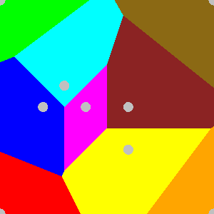
This picture shows us what the Voronoi diagram looks like. Nonetheless, information technology doesn't actually work out the shape of the diagram. Instead, it simply discretizes the region, so looks at each pixel and asks which generator is closest. In some ways, the program looks smarter than it is!
PLOT_POINTS - A Skimpy only Verbal Film
For our next plot, let's use the program PLOT_POINTS. This is an interactive program. We'll keep the interaction brusk though:
plot_points diamond_02_00009.xy voronoi quitIf we didn't include the input file name on the command line, we could have indicated it straight to the program by a command like
read diamond_02_00009.xyThe voronoi command tells the program to compute the Voronoi diagram and save it to an Encapsulated PostScript file; I used convert to plow information technology into a PNG file.
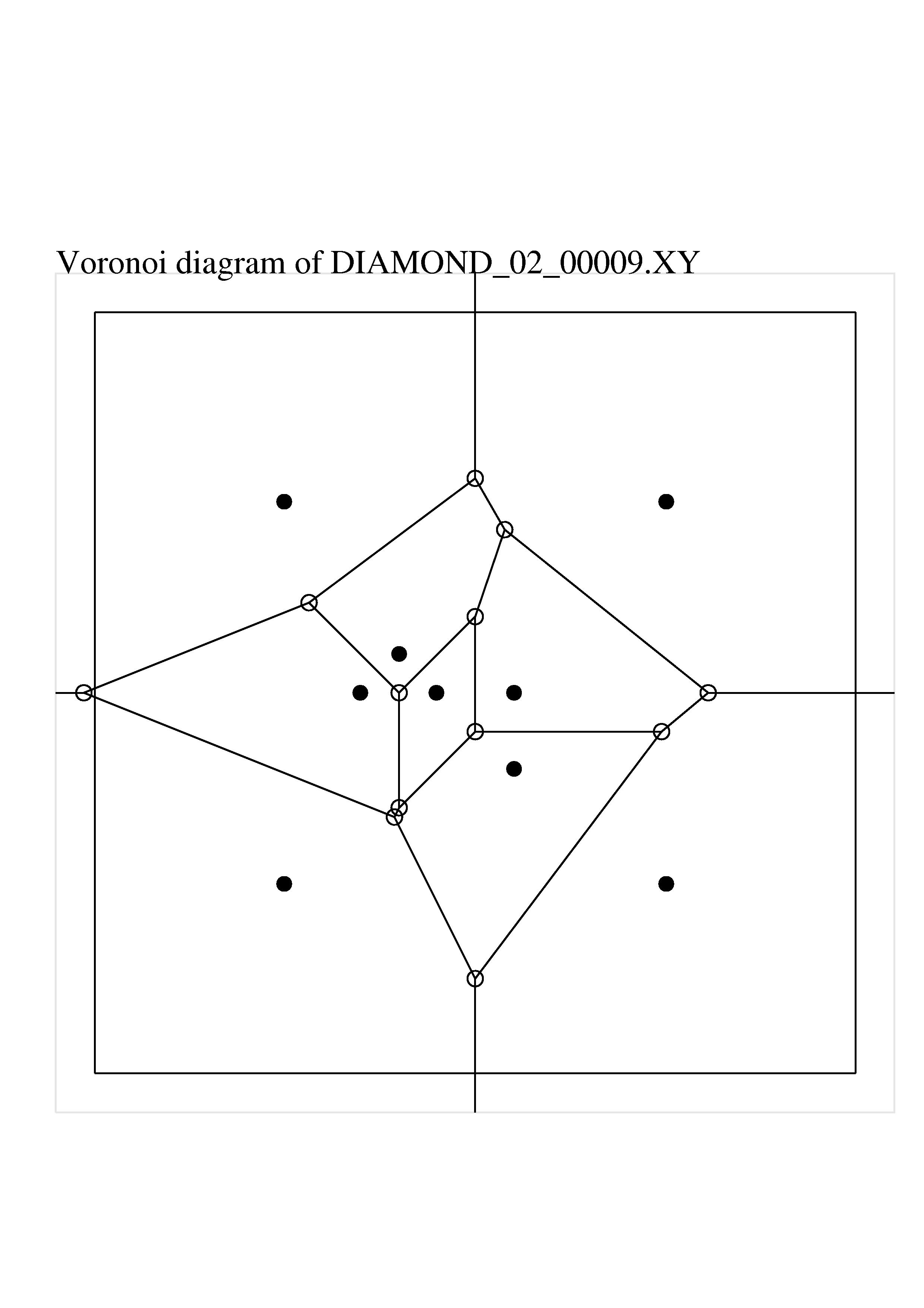
Actually, in society to become the plan to include a larger area, I likewise gave the input control
box -0.five, -0.5, one.5, 1.5This is because I wanted to be sure the program demonstrated that it knows virtually, and can draw, the parts of the Voronoi diagram that extend to infinity.
This picture show is less attractive than the one created past VORONOI_PLOT. Still, notice that this plan must be considerably smarter. The open up circles signal the location of Voronoi vertices, which the programme must take worked out. It also must take worked out where the boundaries of the Voronoi diagram were. Information technology besides knows almost, and handles correctly, the semi-space rays that are role of the Voronoi diagram of the generators that prevarication on the convex hull of the pointset.
It'south not actually articulate from this plot whether the program "knows" the sequence of Voronoi vertices that surround each generator. It could just have a list of the line segments and rays that make upwardly the diagram, which is enough to depict the flick (our centre takes care of figuring out the relationship between the generators and the vertices). However, for many applications, we will need to know the Voronoi vertex sequence, along with the complications that occur when a Voronoi region has semi-infinite sides.
I wrote the PLOT_POINTS program, but PLOT_POINTS relies for its Voronoi calculations on another program, which I didn't write, called GEOMPACK, which we'll get to somewhen!
MATHEMATICA'Due south VoronoiDiagram
The Mathematica program includes a detached mathematics package that can compute Voronoi diagrams. The following commands ready our data. (Note that we have to use names similar gxy rather than g_xy because Mathematica uses the underscore character for other purposes!)
Clear[ points ] Needs[ "DiscreteMath`ComputationalGeometry`" ] gxy = { {0.0,0.0}, {0.0,i.0}, {0.2,0.five}, {0.iii,0.6}, {0.iv,0.5}, {0.6,0.iii}, {0.6,0.5}, {one.0,0.0}, {1.0,ane.0} } ListPlot [ gxy, PlotJoined->False ] { vxy, gface } = VoronoiDiagram [ gxy ] Hither, the vxy assortment contains a listing of objects, about of which are 2D coordinates, but a few of which (listed at the stop) are actually infinite rays. The rays are described by the point where the ray starts, and a point further along the ray.
{ {-0.525, 0.500}, { 0.064, 0.735}, { 0.287, 0.175}, { 0.300, 0.200}, { 0.300, 0.500}, { 0.500, -0.250}, { 0.500, 0.400}, { 0.500, 1.062}, { 0.500, 0.700}, { 0.576, 0.928}, { 0.987, 0.400}, { 1.112, 0.500}, Ray[{-0.525, 0.500}, {-i.525, 0.500}], Ray[{ 0.500,-0.250}, { 0.500,-ane.250}], Ray[{ 0.500, ane.062}, { 0.500, 2.062}], Ray[{ one.112, 0.500}, { 2.112, 0.500}] } Each entry of the gface array contains the alphabetize of a generator (one of the original points), and the indices of the entries in vxy that grade the Voronoi polygon around that generator. The actual class of gface returned is:
{ { 1, { half dozen, 3, i,13,14} }, { two, { 1, 2, 8,15,13} }, { 3, { one, iii, 4, 5, ii} }, { iv, { 2, five, 9,10, viii} }, { 5, { 5, 4, vii, 9} }, { 6, { 4, 3, half dozen,11, seven} }, { 7, { nine, seven,11,12,10} }, { 8, { 12,11, half-dozen,14,16} }, { ix, { 8,10,12,16,15} } } In order to get a plot of the information computed by VoronoiDiagram, we issue a command like this:
DiagramPlot [ gxy, vxy, gface ]which will result in an image similar this:
Thus, with a trivial Mathematica savvy, it is possible to describe a particular Voronoi polygon, decide if information technology is finite, find its centroid, and and so on. This is the kind of information nosotros want to know!
MATLAB's VORONOI: A Plot With Shortcomings!
The MATLAB program is a very handy interactive program. Information technology includes a number of computational geometry routines, and in detail, a voronoi command that makes the kind of plot nosotros're interested in. With an eye to future work, permit'south first see if we tin can somehow get the information in the DIAMOND file into MATLAB. One mode to do this is to employ the MATLAB versions of the TABLE_READ routine. If we've copied the file table_read.chiliad, then we tin can tell MATLAB to get our file as follows:
g_xy = table_read ( 'diamond_02_00009.xy' );Then nosotros can make a Voronoi plot easily with the command
voronoi ( g_xy(:,1), g_xy(:,2) );The result tin can exist exported directly from MATLAB to a JPEG file, and looks something like this:

Although MATLAB is flexible, fast, and piece of cake to use, the output of the VORONOI command isn't quite what we want. First of all, we're only getting a picture, not information. And in fact, if y'all save the output of the control:
[ l_x, l_y ] = voronoi ( g_x, g_y );you get but a set of data describing the line segments to be drawn. In other words, l_x is an array of 2 rows and l_num columns, where l_num is the number of (finite) line segments in the Voronoi diagram.
Thus, although the voronoi control plots the diagram, we could do this ourselves via the commands:
[ l_x, l_y ] = voronoi ( g_x, g_y ); [ dummy, l_num ] = size ( l_x ); for ( l = i : l_num ) plot ( l_x(one:2,l), l_y(one:2,l) ) finish
But if nosotros're interested in how the line segments are grouped to make polygons, we're out of luck. There is no information returned by the command.
One drawback of the voronoi control is that, by default, it frames the plot within the convex hull of the original set of points. This means, specially for small point sets, that a fair chunk of the interesting part of the picture is not shown, including some Voronoi vertices.
Moreover, the Voronoi diagram always includes some semi-space sides, but the voronoi control does not compute or plot these. If the semi-space edges aren't drawn, you miss some important aspects of the motion-picture show.
In order to address these problems, information technology is necessary to work with a more sophisticated MATLAB command called voronoin.
MATLAB'southward VORONOIN: Plots and Information
For serious applications (including datasets in 3D or college dimension), MATLAB includes a more general function called VORONOIN.
[ v_xy, g_face ] = voronoin( g_xy )At present v_xy is a list of vertex coordinates, and the I-th entry of the vector prison cell-assortment g_face is a list of the indices of Voronoi vertices (whose coordinates are in v_xy) that comprise the Voronoi polygon around the I-th generator.
Because g_face is non a simple matrix, it may exist of interest to come across how to display the entries:
for ( i = 1 : length ( g_face ) ) disp ( g_face{i} ); finish (Note that g_face is indexed by curly braces!) For 2d bug, the vertices in g_face are listed in adjacent guild. Thus, continuing this example, nosotros could display the 3rd Voronoi cell by extracting the 3rd row of g_face, using information technology to index v_xy and drawing the convex hull of the result:
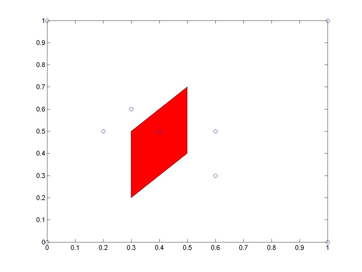
v3_x = v_xy ( g_face{3}, 1 ); v3_y = v_xy ( g_face{3}, ii ); one thousand = convhull ( v3_x, v3_y ); plot ( v3_x(k), v3_y(k) ); If we replace the plot command past a fill command to create a filled polygon, and add a scatter command to display the original points, we can see a plot of the private Voronoi jail cell:
fill up ( v3_x(k), v3_y(m), 'r' ); hold on; besprinkle ( g_xy(1,:), g_xy(ii,:) );
Unfortunately, in that location is not enough data provided in the v_xy and g_face to take care of the semi-infinite Voronoi regions. All we are told in g_face is that such polygons begin and end with the same unmarried betoken at infinity. While this tells us something (the polygon is semi-infinite), information technology does not tell us how to draw the ray that denotes the boundary between this semi-infinite polygon and its (as well semi-infinite) neighbour.
The online MATLAB documentation for VORONOIN claims that it is delivering this data from an internal copy of the QHULL plan, and that assist with the semi-infinite ray directions can be gotten by adding an advisable parameter, but this "documentation" has failed to assist me! My few attempts to effigy out where this information is hidden have brought nothing and then far.
Fortune's SWEEP2
Steve Fortune wrote a C plan called SWEEP2 which tin produce the Voronoi diagram or Delaunay triangulation of a set of points. To compute the Voronoi triangulation, the point fix must exist in a file, say points.txt, with each line containing the coordinates of a single point. Issuing the command
sweep2 < points.txt > points_del.txtwill create an output file containing information defining the Voronoi diagram.
The clarification of the Voronoi diagram is fairly complicated. In that location are four kinds of records in the output file:
- s x y
indicates an input point (or "site") at (x,y); - 5 x y
indicates a Voronoi vertex at the point (10,y); - l a b c
indicates a line with the equation a*x+b*y=c. These lines are non actually drawn, simply are used in the description of the next object; - e fifty v1 v2
indicates a Voronoi edge, which is the segment of the line with index 50 that extends from Voronoi vertex v1 to v2. If either vertex has the value -i, this indicates that the line segment is actually a semi-infinite ray, which extends to infinity on that side;
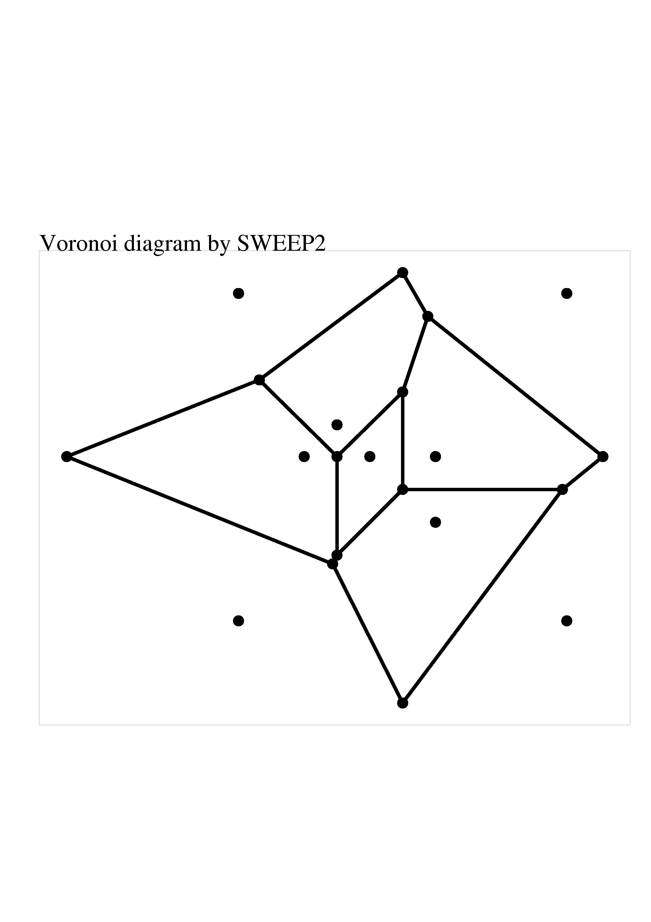
For the diamond dataset, the SWEEP2 plan produced the output file:
southward 0.000000 0.000000 s 1.000000 0.000000 l 1.000000 0.000000 0.500000 southward 0.600000 0.300000 l 1.000000 -0.750000 0.687500 v 0.500000 -0.250000 fifty 1.000000 0.500000 0.375000 s 0.200000 0.500000 50 0.400000 i.000000 0.290000 s 0.400000 0.500000 l 1.000000 -1.000000 0.100000 s 0.600000 0.500000 fifty 0.000000 ane.000000 0.400000 5 0.287500 0.175000 e 2 one 0 l 1.000000 -0.500000 0.200000 v 0.300000 0.200000 eastward vi 1 two fifty 1.000000 0.000000 0.300000 v 0.500000 0.400000 e 4 2 3 l one.000000 0.000000 0.500000 south 0.300000 0.600000 l 1.000000 one.000000 0.800000 v 0.300000 0.500000 eastward 7 4 2 50 -1.000000 ane.000000 0.200000 v 0.987500 0.400000 e 5 three v e 1 0 5 l -0.800000 1.000000 -0.390000 five 0.500000 0.700000 east 10 4 half-dozen e 8 half-dozen three 50 1.000000 -0.333333 0.266667 s 0.000000 i.000000 fifty -0.400000 i.000000 0.710000 s ane.000000 1.000000 l 0.800000 ane.000000 one.390000 v 0.064286 0.735714 e 9 7 4 l -0.750000 1.000000 0.687500 v i.112500 0.500000 e eleven 5 8 50 0.000000 1.000000 0.500000 v -0.525000 0.500000 east 3 9 ane e xiii 9 seven 50 0.000000 1.000000 0.500000 v 0.576316 0.928947 east 12 vi ten e 14 10 8 l 1.000000 0.571429 1.107143 five 0.500000 i.062500 e fifteen 7 11 e 18 eleven 10 fifty 1.000000 0.000000 0.500000 eastward 17 -1 nine e 19 -1 11 east 16 8 -1 e 0 0 -1
The output from the SWEEP2 may seem excessive and obscure, but it has some very interesting properties. Permit usa begin by noting that the s records in the output practise non occur in the aforementioned lodge every bit they were input. They have been sorted by the y coordinate:
#0: s 0.000000 0.000000 #1: s 1.000000 0.000000 #2: southward 0.600000 0.300000 #iii: s 0.200000 0.500000 #4: s 0.400000 0.500000 #5: s 0.600000 0.500000 #6: southward 0.300000 0.600000 #7: s 0.000000 one.000000 #8: s i.000000 1.000000Now notice that, after the first two sites have been output, the next detail in the file is a "line" object,
l 1.000000 0.000000 0.500000which indicates that line #0 has the equation
one.0 * x + 0.0 * y = 0.vwhich is the perpendicular bisector of the line between sites #0 and #1. The program has really just considered the get-go ii points, and now "knows" that it may need the perpendicular bisector between them.
Afterwards reading another site, it outputs line #ane, so outputs Voronoi vertex #0. The reason that the code can output this Voronoi vertex is that it knows the points have been sorted by y coordinate, and so office of the Voronoi diagram is actually now mainly understood. It turns out that you can be certain of the location of Voronoi vertices sooner than you can be sure of the extent of Voronoi edges, (partly considering you have to know where ii vertices are to specify one edge), so it's not until six sites have been processed, and 2 vertices determined, that nosotros can determine the first Voronoi edge. (And in some examples, information technology might be the case that many Voronoi vertices would be determined before even one Voronoi edge could exist ready.)
This incremental arroyo to processing the data keeps the internal retentiveness requirements depression and speeds the algorithm. Of course, information technology also explains why the output of the iv kinds of records occurs in a jumble, as y'all go.
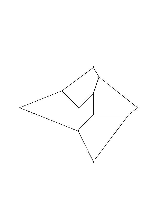
I have drafted a program SWEEP2_VORONOI_EPS, which is able to read the Voronoi diagram information, and construct an Encapsulated PostScript file containing an image of the diagram. The program has a few flaws. Although SWEEP2's information file does include information about the semi-space Voronoi edges, I take not nevertheless washed the work necessary to draw them. And the plot by default includes all points and vertices, and so the SWEEP2 test dataset does not have a very nice plot, because the data is entirely in the unit foursquare, except for a single vertex with x coordinate -13. This causes the plot to be very badly scaled.
Here is the Voronoi plot created for the diamond data prepare:
Barry Joe's GEOMPACK
Barry Joe wrote several versions of a FORTRAN package chosen GEOMPACK, which computes the Voronoi diagram or Delaunay triangulation using fairly uncomplicated data types. Most versions of the package contain many more routines than you demand. The central routine is called either DTRIS or DTRIS2 or RTRIS or RTRIS2; the D or R was used to distinguish double and single precision versions, and the ii was used after Barry Joe developed 3D versions of the code as well.
I have a version of this program, which I converted to FORTRAN90, in the directory ../f_src/geompack/geompack.html
I have a 2nd version of a subset of this plan, which I converted to C++, in the directory ../../cpp_src/geompack/geompack.html While information technology is much less all-encompassing than the FORTRAN version, information technology includes the RTRIS2 routine, and and so can do a Delaunay triangulation.
The RTRIS2 lawmaking computes the Delaunay triangulation directly from the coordinates of a point set.
The RTRIS2 code computes the Delaunay triangulation, but not the Voronoi diagram. However, since these ii objects are so closely related, it is possible to get from 1 to the other. I did this one time already in PLOT_POINTS, and hither will sketch out what has to be done.
Start with g_num points with coordinates in g_xy. To generate the Delaunay triangulation, we call
telephone call rtris2 ( g_num, g_xy, v_num, nod_tri, tnbr )
Alarm! It is important to note that RTRIS2, as written, sorts the betoken coordinates, and on exit, returns the sorted point coordinates. This can be very disruptive if you are non enlightened of it! I find this fact so unpleasant that, in many cases, I take modified RTRIS2 so that it works with an index sort vector instead, producing the same output as earlier, except that the point coordinates are not modified. Before I made this modify, I repeatedly encountered severe problems, such as making a plot using the old node coordinates, just with triangulation data that assumed the node coordinates had been shuffled by the sorting. The upshot is a meaningless spaghetti plot! And this hardens my belief that a subroutine's arguments should be INPUT or OUTPUT but Not both!
Interpreting the output of RTRIS2
The number of Voronoi vertices (and Delaunay triangles) is returned every bit v_num; for our sample problem, this value is v_num=12.
The assortment nod_tri(1:three,v_num) lists the 3 generators that grade the vertices of each Delaunay triangle; for our sample problem, this array looks like:
1 ii 1 3 2 3 ane 6 3 2 three 4 iv four three five v 7 4 5 six 5 3 vi vii 7 v 6 8 9 4 7 9 6 i 8 10 7 6 8 11 7 8 ix 12 2 four 9
The assortment tnbr indicates, for each Delaunay triangle (or Voronoi vertex) the alphabetize of the neighboring triangle (or vertex) along each side. However, some triangles don't have a neighbour on a particular side (and correspondingly, some Voronoi vertices don't take a finite Voronoi neighbour). In such cases, the respective entry is a negative value:
1 -i two 3 2 i 9 6 3 i 4 12 4 three half-dozen 5 5 8 iv 7 half-dozen iv 2 vii vii v 6 10 8 12 v 11 ix 2 -2 10 10 7 9 eleven 11 10 -3 viii 12 3 viii -four(The actual negative values returned by RTRIS2 are different, and somewhat arbitrary. I've made them consecutive for simplicity.)
Can we get Voronoi information from RTRIS2?
This is the data nosotros are going to have to manipulate in social club to determine the Voronoi data.
The easiest thing to do is to compute the circumcenter of each Delaunay triangle, because these are the vertices of the Voronoi polygons!
do v = ane, v_num call triangle_circumcenter_2d ( g_xy(1,nod_tri(1,v)), g_xy(two,nod_tri(1,5)), g_xy(1,nod_tri(two,five)), g_xy(2,nod_tri(ii,five)), g_xy(1,nod_tri(3,v)), g_xy(2,nod_tri(three,v)), v_xy(1,5), v_xy(2,five) ) end exercise
Now, to describe the Voronoi diagram, wait at each Delaunay triangle, and each border of that Delaunay triangle. If there is a neighboring triangle along that border, then connect the 2 circumcenters. If there is no neighbor, then this is an infinite edge, so yous tin extend a line indefinitely from the circumcenter through that side in the outward normal direction.
do v = 1, v_num do j = 1, 3 one thousand = tnbr(j,v) if ( 0 < chiliad ) and so connect v_xy(1:2,v) to v_xy(1:2,k) else decide outward normal North to the triangle edge, and depict a ray from v_xy(1:ii,v) end if stop do end do
Going through this procedure now, I retrieve that information technology took me a long time to work it out from the data that GEOMPACK supplies. As well, I realize that we don't actually accept a convenient data structure that lists the Voronoi vertices that course a detail Voronoi diagram. You'd have to examine every Delaunay triangle and run into whether your node of interest was ane of the three vertices of the triangle. The index of that triangle is also the index of the circumcenter. From that triangle, y'all can look to the "left" and "right" to detect the previous and side by side vertices in the Voronoi polygon, and thus either go all the manner around a finite polygon, or come to the ends of an infinite one. Well, it'south doable, just I didn't do information technology!
Versions of RTRIS2
As mentioned above, RTRIS2 and its underlying routines are bachelor in the FORTRAN90 code GEOMPACK. I have also extracted these routines for use in the PLOT_POINTS program, in order to compute and display Delaunay triangulations and Voronoi diagrams.
I likewise put a re-create of the routines in the FORTRAN90 GEOMETRY library, forth with many routines for printing out the arrays associated with the triangulation. The exam lawmaking for GEOMETRY includes a setup of the DIAMOND dataset.
I have merely recently worked out a C++ version of RTRIS2, made bachelor in the C++ GEOMETRY library. This does not yet include the extra routines for printing out the triangulation arrays The test code includes a setup of the DIAMOND dataset.
TABLE_VORONOI
I decided that nosotros needed a good FORTRAN code that returns the Voronoi diagram data. I based the code on the RTRIS2 routines from GEOMPACK, and used the ideas that had worked in PLOT_POINTS to convert the Delaunay information to Voronoi data. Nonetheless, PLOT_POINTS was only cartoon a picture, so it didn't need to be construct a full information construction description of the Voronoi diagram. For my purposes, I needed to figure out a data construction that would encapsulate the Voronoi diagram, and allow me not only to plot the diagram, just to record all the polygonal degree and neighbor information. If this was done properly, then information technology would exist easy, for example, to determine if any Voronoi cell was finite, and to compute the area or centroid of any finite cell.
The program is interactive. It assumes that the user has prepared a listing of the point coordinates, in the form of an XY data file, so that the program invocation looks something like
table_voronoi diamond.xy
The plan counts g_num, the number of generators, and stores the coordinates in the assortment g_xy(1:2,one:g_num). The program then calls GEOMPACK to compute the Delaunay triangulation, and from that data computes the post-obit Voronoi quantities:
- g_degree, for generator 1000, the degree of the Voronoi polygon;
- g_start, for generator Grand, the index of the outset Voronoi vertex in a traversal of the Voronoi polygon;
- g_face, for all generators One thousand, a listing of the Voronoi vertices in a traversal of the Voronoi polygon;
- v_num, the number of Voronoi vertices;
- v_xy, for each Voronoi vertex Five, the XY coordinates.
- i_num, the number of Voronoi vertices "at infinity";
- i_xy, the directions of the Voronoi vertices at infinity.
For our sample problem, the information for the g_num=9 generators is:
1000 G_DEGREE G_START G_FACE one 5 1 -14 nine 2 one -13 2 v 4 -thirteen 1 three 12 -16 three 5 seven 1 3 4 six 2 4 5 12 3 12 8 v 4 5 4 17 iv v 7 vi 6 5 21 2 6 vii 10 nine 7 5 26 5 eight eleven 10 7 8 5 31 -15 xi 10 9 -14 nine 5 34 -16 12 viii 11 -fifteenHere, the negative entries betoken fictitious nodes at infinity, whose directions are stored in i_xy. For the v_num=12 Voronoi vertices,
Five V_XY i -0.525 0.500 2 0.287 0.175 3 0.064 0.735 4 0.300 0.500 v 0.500 0.700 half-dozen 0.300 0.200 7 0.500 0.400 eight 0.576 0.928 nine 0.500 -0.250 10 0.987 0.400 xi ane.112 0.500 12 0.500 1.062and, with i_num = 4, the "directions" of the fictitious nodes at infinity are
I I_XY 1 -1.0 0.0 2 0.0 -1.0 3 1.0 0.0 4 0.0 i.0(You could also relabel the fictious nodes at infinity with the values xiii, 14, 15 and 16, and stick the four values in I_XY onto the end of the V_XY array, if you could keep clear that these four values are actually directions, not locations!)
Annotation that, to describe the rays that form office of the boundary of the unbounded regions, you look for a negative node in G_FACE. Suppose we are working on the region associated with the first generator. And so the starting time negative index we encounter is -14. Make it positive, and decrease the value of V_NUM to become its index of ii. This gets you the direction (0.0,-i.0) in the I_XY array.
Now look for the predecessor or successor of 14 in the G_FACE array (Negative entries only occur as the start or last entries in a list). In this case, -14 is followed by nine. And so to draw this portion of the purlieus, you start at node ix, and draw as much of the direction
( v_xy(1,9) + s * i_xy(1,2), v_xy(two,nine) + s * i_xy(2,ii) )every bit volition fit in your picture. For region one, the other ray is associated with the negative node -13, we movement to its finite predecessor in the list, vertex 1, and draw a line from there in the management stored in I_XY, entry |-13|-12 = 1. At that place, wasn't that easy?
I understand that the ready of data structures and conventions described hither is not the cleanest. It is also true that the method past which I "massage" the Delaunay data coming out of GEOMPACK is inefficient and very slow if the number of generators is big. But I do believe that I've tracked down the information necessary to plot and more importantly analyze the Voronoi regions, including the oftentimes-neglected unbounded regions.
Renka'south TRIPACK and STRIPACK
Robert Renka has published a number of algorithms in ACM TOMS. In particular, TRIPACK (ACM TOMS Algorithm #751) computes the Delaunay triangulation of a prepare of points in the airplane. From the remarks above near GEOMPACK, it should exist articulate that this information is plenty to compute the Voronoi diagram.
Some other algorithm published past Renka is STRIPACK, (ACM TOMS Algorithm #772). This is substantially the aforementioned as TRIPACK, except that the points lie on a sphere. It should (eventually) be clear that the information well-nigh a Delaunay triangulation on a sphere is enough to piece of work out the Voronoi diagram, with the added feature that there are no infinite regions.
Shewchuk's TRIANGLE
TRIANGLE is Jonathan Shewchuk'southward C program for producing meshes, Delaunay triangulations and Voronoi diagrams. Y'all can expect at my local copy of TRIANGLE.
TRIANGLE requires a slightly dissimilar input file from the XY format nosotros have used elsewhere, called the "node" format. The '#' comment lines in our XY format are still acceptable, but at that place must be 1 line that specifies the number of nodes (and some other information) and each line of coordinate information must brainstorm with the index of the vertex. A version of our DIAMOND data looks something like this:
# diamond_02_00009.node nine 2 0 0 1 0.0 0.0 2 0.0 1.0 3 0.2 0.v 4 0.three 0.half dozen 5 0.iv 0.five 6 0.6 0.3 7 0.6 0.5 viii one.0 0.0 9 1.0 1.0
If nosotros now invoke TRIANGLE with the "-five" (for Voronoi) pick:
triangle -v diamond_02_00009.nodeinformation technology rapidly creates four files:
- diamond_02_00009.1.node, the Delaunay nodes;
- diamond_02_00009.i.ele, the Delaunay triangles;
- diamond_02_00009.1.v.node, the Voronoi nodes (vertices);
- diamond_02_00009.i.5.edge, the Voronoi edges (polygon sides);
The file diamond_02_00009.one.five.node corresponds to our data construction g_xy. Information technology includes the four corners of the diamond, so nosotros know that's right:
12 2 0 0 i -0.525 0.500 2 0.300 0.500 three 0.500 1.062 4 0.064 0.735 5 0.287 0.175 six 0.987 0.400 7 0.500 -0.250 eight 0.576 0.928 ix 0.500 0.400 x 1.112 0.500 11 0.500 0.700 12 0.300 0.200 # Generated by triangle -v diamond_02_00009.node(I've reformatted this file so that the data lines up, and is all printed to iii decimals, only to make comparisons easier.)
The file diamond_02_00009.1.5.edge corresponds to our data structure l_vert. However, information technology lists twenty edges, which includes the 4 space edges. These are marked by the use of a format in which the 2nd node index is -1, followed past two values which are interpreted every bit the direction of the infinite ray. Thus, the 9th edge starts at Voronoi vertex iii, and so extends infinitely in the direction (0,i), an upward vertical ray.
xx 0 1 ane 5 2 1 iv three ane -1 -one 0 4 2 4 five ii 12 6 ii 11 seven three 4 8 3 8 ix 3 -i 0 1 ten 5 vii 11 5 12 12 6 7 13 6 ten fourteen six ix 15 seven -1 0 -1 16 8 10 17 8 11 18 9 11 19 ix 12 20 10 -1 one 0 # Generated by triangle -v diamond_02_00009.node
Again, we accept lots of information, but not, apparently, an explicit list of the Voronoi vertices that environment each generator. To determine the Voronoi vertices around node v, then, nosotros need to read the Delaunay triangulation border listing (diamond_02_00009.i.ele) for triangles that include node five, which turns out to be triangles ii, 9, 11, and 12. The corresponding Voronoi vertices are listed in diamond_02_00009.one.five.node. If we really desire to list the vertices in order, to produce a traversal of the polygon, then we demand to look at the Delaunay triangles and find matching pairs of edges.
TRIANGLE includes another program called SHOWME which can be used to make an X-window display of a mesh, or to save an image as a PostScript file.
To encounter the Voronoi diagram we just created, it is only necessary to blazon
showme diamond_02_00009.1.v.edgeI salvage the image as a PostScript file, and converted that to JPEG using GSView.
QVORONOI
The QVORONOI programme is office of the QHULL packet, which has a dwelling folio at http://world wide web.thesa.com/software/qhull/.
QVORONOI is an interactive plan that reads an input file, computes the Delaunay triangulation, determines the Voronoi diagram, and either prints a summary, or outputs the information to a file, based on control line switches.
The format for the pointset coordinate file is fairly simple. Lines kickoff with a nonnumeric graphic symbol are treated as comments. The outset noncomment line must incorporate the spatial dimension; the second line gives the number of points, and each subsequent line lists the coordinates of a single point. Thus, our standard diamond example file would be slightly modified from "xy" format to a new format nosotros could telephone call "qxy", which might look like this:
# diamond_02_00009.qxy # 2 9 0.0 0.0 0.0 1.0 0.ii 0.five 0.three 0.six 0.4 0.5 0.6 0.three 0.6 0.5 1.0 0.0 1.0 1.0
The command line switch "p" requests that the coordinates of the Voronoi vertices be listed (which we've called V_XY). Thus, the command
qvoronoi diamond_02_00009.qxy presults in the output:
2 12 0.500 -0.250 -0.525 0.500 0.287 0.175 0.300 0.200 one.112 0.500 0.987 0.400 0.500 0.400 0.064 0.735 0.300 0.500 0.500 i.062 0.500 0.700 0.576 0.928which nosotros recognize as a proper list of the Voronoi vertices, with the addition of the 2 initial lines that given the dimension and number. (For clarity, I reformatted this data so that it lined upwardly and only listed 3 decimal places.)
The command line switch "FN" requests that, for each generator, the sequence of Voronoi vertices exist listed. Thus, the control
qvoronoi diamond_02_00009.qxy FNresults in the output:
9 4 2 0 -1 1 4 ix -1 1 seven 5 8 iii 2 1 7 v 11 9 seven 8 10 iv 10 half-dozen iii viii 5 6 iii 2 0 five 5 11 4 5 half-dozen x four five 0 -i 4 4 11 4 -1 9where the "9" indicates the number of generators, and, in the subsequent lines, the start value is the number of vertices (what we called G_DEGREE), followed by the list of vertices (which we've called G_FACE). If the region is unbounded, then a single value of -one in the vertex list indicates the vertex at infinity.
Misadventures trying to plot the QVORONOI OFF output
The command line switch "o" requests that an OFF file be created, containing the information well-nigh the Voronoi diagram, and suitable for display by the GEOMVIEW plan. The grade of this OFF file is:
2 13 9 1 -10.101 -10.101 0.500 -0.250 -0.525 0.500 0.287 0.175 0.300 0.200 1.112 0.500 0.987 0.400 0.500 0.400 0.064 0.735 0.300 0.500 0.500 1.062 0.500 0.700 0.576 0.928 4 3 one 0 2 iv 10 0 2 eight v nine 4 3 2 8 5 12 10 8 9 11 4 11 7 4 nine 5 7 4 3 one vi 5 12 v 6 7 eleven four vi 1 0 5 4 12 v 0 tenAbout of this information makes sense. The initial "two" says that the information is two-dimensional. The adjacent line says at that place are 13(?) nodes and ix faces and i(?) border. There are thirteen nodes considering the program adds the bogus point (-x.101, -10.101) as a standin for infinity, and the edges are listed as 1 because this slice of information is no longer used, but a dummy value must exist supplied. Discover that the vertex indices range from 0 to 12, with 0 being the point at infinity.
This data file is supposed to be usable as input to the GEOMVIEW program. All the same, information technology was simply after a sure amount of piece of work that I was able to get the program installed, it did not accept the input file, (the initial "ii" had to be deleted, and a magic "OFF" inserted in that location) and after I "fixed up" the input file, (past calculation a Z coordinate of 0 to each point) the plot was unacceptable; after I massaged the information (by moving the point at "infinity" to zero and removing the point at infinity from all the polygons), I did see the diamond-shaped region, but of class without the space edges. Just when I tried to relieve an re-create of this poor image in PPMA format, the program froze and I had to exit with nix. My initial verdict on viewing QVORONOI OFF files with GEOMVIEW is therefore, don't bother!
TABLE_VORONOI
In some frustration, I spent some time sketching out a program called TABLE_VORONOI to compute plenty information to get the Voronoi diagram correct. What I came upwards with is a program that doesn't actually know how to store this data, but prints it out. That makes it impractical for big calculations; it's simply a kickoff. However, I just didn't accept the time to work out how to set up an array to handle the information, particularly since nosotros're tracking polygons and semi-space polygons of varying degree.
Nonetheless, I was able to run across that the things I wanted are computable.
The program begins with the pointset, of which a typical chemical element is a indicate K. Each G generates a Voronoi polygon (or semi-infinite region, which nosotros will persist in calling a polygon). A typical vertex of the polygon is chosen V. For the semi-space regions, we take a vertex at infinity, only it'due south actually not helpful to store a vertex (Inf,Inf), since we have lost information nearly the direction from which nosotros achieve that infinite vertex. Nosotros will have to treat these special regions with a little extra intendance.
We are interested in computing the following quantities:
- G_DEGREE, for generator G, the degree (number of vertices) of the Voronoi polygon;
- G_START, for generator Grand, the index of the get-go Voronoi vertex in a traversal of the sides of the Voronoi polygon;
- G_FACE, for all generators G, the sequence of Voronoi vertices in a traversal of the sides of the Voronoi polygon. A traversal of a semi-space polygon begins at an "space" vertex, lists the finite vertices, and then ends with a (different) infinite vertex. Infinite vertices are given negative indexes.
- V_NUM, the number of (finite) Voronoi vertices V;
- V_XY, for each finite Voronoi vertex Five, the XY coordinates.
- I_NUM, the number of Voronoi vertices at infinity;
- I_XY, the "direction" associated with each Voronoi vertex at infinity.
So if we accept to draw a semi-infinite region, we start at infinity. Nosotros then need to draw a line from infinity to vertex #2. We practise so by drawing a line in the appropriate direction, stored in I_XY. Having safely reached finite vertex #2, we can connect the finite vertices, until information technology is time to draw some other line to infinity, this time in another direction, also stored in I_XY.
Considerations for the CVT Iteration
A Centroidal Voronoi Tessellation (CVT) is a set of generators with the special property that each generator is the centroid of its Voronoi cell. It is not easy in general to compute a CVT; in that location is an implicit relationship between the location of the generators and the shape of their Voronoi regions. However, a CVT with a given number of generators, confined to a given region, can be approximated by one of several kinds of iterations. Aside from requiring a divisional region, some iterations likewise need to compute the surface area and centroids of the Voronoi cells. Other iterations are probabilistic, and can judge these quantities using sampling.
The bounded region
For a CVT calculation, we normally assume that the generators and all the points of involvement are restricted to a finite bounding region. Nosotros tin can notwithstanding generate the total Voronoi diagram, with some space cells, just nosotros simply consider the intersection of this diagram with the bounding region. Since each generator is within the bounding region, or at least on its boundary, and finitely separated from all other generators, it volition never have an empty Voronoi cell, fifty-fifty after we discard the part outside the bounding region.
The bounding box is crucial because, equally part of the computation, we need to compute the centroids of the individual Voronoi cells. If the region is space, then some of our centroids will also exist infinite and the algorithm will break downwardly. The fact that each generator'southward Voronoi jail cell volition have some positive area within the bounding region also keeps the algorithm operating smoothly.
The exact CVT methods require the explicit structure of the Voronoi cells, and the ciphering of their areas and centroids. If the region were infinite, then the Voronoi cells would always accept polygonal sides, so the expanse and centroid calculations are easy. But with a bounding region, we now face the situtation that some Voronoi cells will have the boundary of the region as i of their sides. If the shape of this bounding bend is arbitrary, then nosotros may accept a difficult time determining the shape, surface area, and centroid of the corresponding Voronoi cell. For convenience, let the states presume that the bounding region itself is polygonal. Nosotros might farther assume that it is convex, or has sides that are always forth coordinate directions. In the simplest instance, we may assume that the bounding region is actually an M-dimensional interval, or generalized box.
In this simplest case of an Thousand-dimensional interval for the bounding region, it is usually possible to make up one's mind the shape of the intersection of whatever Voronoi cell with the bounding region. For example, in ii dimensions, the shape of such a Voronoi cell can easily be plotted. We simply start with the line segment or semi-space ray that forms one side of the cell. Nosotros then consider each side of the bounding box, and inquire whether the given segment or ray intersects that side. If it does, and then we demand to modify the line segment or ray accordingly, by chopping off any portion that extends past that side of the box. In one case all iv (or ii*M in general) sides of the box accept been considered, nosotros can draw what's left of the line segment or ray.
The program PLOT_POINTS uses this simple method in club to display the portion of a Voronoi diagram that will fit in the current plot box.
Information technology's actually a picayune harder to compute the area of the cell, rather than only to draw it. To practise so, nosotros consider the fact that (at least for our simple cases) the bounding box is convex, and the (original, unbounded) Voronoi cell will be convex, and then the intersection of these two will also be convex. This means we tin can find the shape of the Voronoi cell by starting with the bounding region, and then taking its intersection with the halfplanes defined by each of the bounding lines of the original Voronoi jail cell. Once you remember of the problem this manner, you should be able to organize the adding and the data structure that you would need. Since nosotros stop up with a polygonal region, we know that our trouble is reduced to determining the surface area and centroid of a polygonal region.
The CVT Iteration
There are several iterative procedures that tin can be used to compute a CVT. They each begin from some initial set of generators that lie in the region. In each step of the iteration,
- compute the verbal or approximate Voronoi diagram of the current set of generators;
- compute the verbal or approximate centroid of each Voronoi cell;
- supercede the previous generators by the centroids.
The Exact Version of the CVT Iteration in Depression Dimensions
In 2d, it is possible to behave out each step of this procedure in what is essentially an exact manner. (We're saying here that each footstep of the iterative procedure may be done in an verbal style. Each step nonetheless will produce only an approximation of a CVT. We're only saying that by post-obit this procedure, nosotros'll have made the best approximation that is possible.)
What we are saying is that, given a gear up of generators, it is possible to make up one's mind the location of the Voronoi vertices precisely, to restrict the Voronoi cells to the given finite region, and, assuming the finite region did not introduce any complexity to the shape of the cells, to compute the area and commencement moments of the Voronoi cells, thus arriving at the centroids.
It is also possible, when using some programs, and with rather more overhead, to carry out this process in 3D as well. There are some programs that will compute the organisation of vertices and polygonal faces that form each Voronoi polyhedron. Because of the complexities of 3D geometry, it could be a bit more difficult than in the 2nd case to decide the course of the Voronoi cells when restricting them to the finite region of interest. If these cells remain polyhedra, then it is possible to compute the volume and first moments of the Voronoi cells, thus arriving at the centroid.
In college dimensions, information technology is not really feasible to pursue this exact approach, and instead, approaches using probablistic sampling must be applied in order to estimate the volume and centroid and carry out each pace of the CVT iteration.
Withal, the 2nd and 3D cases are fairly common, then information technology should be of interest to note how one can compute areas, volumes and centroids. These matters are now briefly considered.
The Surface area of a (Polygonal) Voronoi Cell in 2D
In 2D, the surface area of a polygon P with N vertices is easy to compute. We assume we are given the coordinates of the vertices, and we may presume that the polygon is non degenerate (in particular, that the polygon is non folded over on itself.)
The simplest approach is to triangulate the polygon and add together up the areas; if we aren't particular, we tin cull vertex Due north as the base of operations, and then consider the N-2 triangles formed by the base vertex plus consecutive pairs of vertices from (i,2) through (N-2,N-i):
Area ( P ) = sum ( T in P ) area ( T )where the area of a triangle is easily computed:
Surface area ( T ) = i/2 * ( x1 * ( y2 - y3 ) + x2 * ( y3 - y1 ) + x3 * ( y1 - y2 ) )(In the formula for the triangle, the indices 1, 2, and three just indicate the iii vertices of the triangle, and don't refer to the original numbering of the vertices of the polygon.)
A 2nd formula for polygonal expanse is only
Expanse ( P ) = 1/ii * sum ( 1 <= i <= Northward ) 10(i) * ( y(i+i) - y(i-1) )where we "wrap around" the indices when they exceed the legal range.
In MATLAB, if the coordinates of a polygon are stored in the cavalcade vectors p_x and p_y, then the area of the polygon can exist plant with the command
area = polyarea ( p_x, p_y )
In some cases, instead of having the vertices of the Voronoi polygon around generator K, we might take the list of generators that are Delaunay neighbors. This is really a fairly common situation. It is nevertheless possible to compute the expanse of the Voronoi polygon directly from this data, using a formula given in Spatial Tesselations [Okabe].
The Centroid of a (Polygonal) Voronoi Prison cell in 2nd
The x coordinate of the centroid of a 2d region P is
centroid_x ( P )= Integral ( 10, y in S ) ten dx dy / Area ( P )with the y coordinate of the centroid divers similarly.
One approach to computing the centroid of a Voronoi cell in 2d is simply to compute the areas and centroids of the component triangles (again, choosing an arbitrary base signal to use in triangulation). We already know how to compute the expanse of a triangle. The centroid of a triangle is simply the average of the iii vertices:
centroid ( T ) = ( (x1,y1) + (x2,y2) + (x3,y3) ) / 3And then the centroid of the polygon is found by adding upward the centroids of the component triangles, each weighted by its area, and dividing by the sum of the areas of the triangles.
centroid ( P ) = sum ( T in P ) area ( T ) * centroid ( T ) / sum ( T in P ) expanse ( T )
A second formula, for the X component of the centroid of the polygon, is
centroid_x ( P ) = 1/half dozen * sum ( ane <= i <= N ) ( ten(i+1) + x(i) ) * ( x(i) * y(i+1) - 10(i+1) * y(i) ) ) / Area ( P )with a similar formula for the Y component.
Now suppose that instead of having the vertices of the Voronoi polygon around generator G, nosotros have the list of neighbor generators. It is possible to compute the centroid of the Voronoi polygon directly from this data, using a formula given in Spatial Tesselations [Okabe].
The formulas for the centroid of a polygon given its vertices, or of a Voronoi cell given the sequence of Delaunay neighbors, are implemented in the GEOMETRY library.
The Vertices of a (Polygonal) Voronoi Jail cell in 2d
Assuming we are only given the Delaunay data about a (finite) Voronoi jail cell, then we know we can draw a flick of the Voronoi polygon, because nosotros simply draw the perpendicular bisector line between the primal node and all its Delaunay neighbors. So the information is in that location. But to analyze the polygon, we actually want to know the coordinates of its vertices.
The cardinal is the fact that each Delaunay triangle corresponds to a Voronoi vertex, and that the Voronoi vertex is the circumcenter of the Delaunay triangle. The circumcenter of a (nondegenerate) triangle is the center of the unique circle which passes through all three nodes.
The formula for coordinates (xc,yc) of the circumcenter depends on the fact that the vectors (x2-x1,y2-y1) and (x3-x1,y3-y1) are secants of the circumvolve. Hence, each secant vector can be used to form a correct triangle along with the diameter vector. Hence, in particular, the dot product of P12 = (x2-x1,y2-y1) with the diameter vector is equal to the squared length of P12, and similarly for P13. Nosotros terminate up having to solve the linear system:
(x2-x1) * xc + (y2-y1) * yc = (x2-x1)**ii + (y2-y1)**2 (x3-x1) * 90 + (y3-y1) * yc = (x3-x1)**ii + (y3-y1)**2to determine the circumcenter. Doing this for each Delaunay triangle gives us the Voronoi vertices.
The Volume of a (Polyhedral) Voronoi Jail cell in 3D
Suppose that we decompose each face F of the polyhedron P into triangles T. Then the book of the polyhedron tin can be found past adding upwards the following terms:
Volume ( P ) = Sum ( F in P ) Sum ( T in F ) ane/6 * ( x1 * y2 * z3 - x1 * y3 * z2 + x2 * y3 * z1 - x2 * y1 * z3 + x3 * y1 * z2 - x3 * y2 * z1 )where the coordinates of the get-go vertex of triangle T are (x1,y1,z1), and so on.
The Centroid of a (Polyhedral) Voronoi Cell in 3D
In gild to compute the centroid of a polyhedron, we first choice a base bespeak somewhere within the polyhedron. Then we pause each polygonal face into triangles. Then, on each triangle, nosotros raise a tetrahedron to the base point. Now the polyhedron has been dissected into disjoint tetrahedrons.
It's easy to compute the volume of each tetrahedron. It'southward even easier to compute the centroid of each tetrahedron, since that'southward simply the boilerplate of its iv vertices. But then it'south uncomplicated to compute the centroid of the polyhedron, because that is but the book-weighted sum of the centroids of the constituent tetrahedrons:
centroid ( P ) = sum ( T in P ) volume ( T ) * centroid ( T ) / sum ( T in P ) book ( T )
The Vertices of a (Polygonal) Voronoi Cell in 3D
In illustration to the 2d case, if nosotros are given Delaunay data nearly a 3d "triangulation" of the region, we have a list of the Delaunay neighbor nodes. If nosotros are careful, we can figure out all the sets of iii neighbour nodes that, along with the eye node, class a Delaunay tetrahedron.
As before, each Delaunay tetrahedron corresponds to a Voronoi vertex, and the Voronoi vertex is again the circumcenter of the Delaunay tetrahedron, which is at present the center of the unique sphere which passes through all four nodes.
The formula for coordinates (xc,yc,zc) of the circumcenter depends on the fact that the vectors such as P12 = (x2-x1,y2-y1,z2-z1) are secants of the sphere. We end upwards having to solve the linear system:
(x2-x1) * xc + (y2-y1) * yc + ( z2-z1) * zc = (x2-x1)**ii + (y2-y1)**2 + (z2-z1)**two (x3-x1) * xc + (y3-y1) * yc + ( z3-z1) * zc = (x3-x1)**ii + (y3-y1)**2 + (z3-z1)**2 (x4-x1) * 90 + (y4-y1) * yc + ( z4-z1) * zc = (x4-x1)**2 + (y4-y1)**2 + (z4-z1)**2to determine the circumcenter. Doing this for each Delaunay tetrahedron gives us the vertices of the Voronoi polyhedron.
The GEOMETRY Library
The formulas for the area and centroid of a polygon in second, the volume and centroid of a polyhedron in 3D, the circumcenter of a triangle in second or tetrahedron in 3D, or the area, centroid and vertices of a Voronoi polygon in 2D given the Delaunay neighbors, are all implemented in the routines:
- POLYGON_AREA_2D computes the area of a polygon in 2d;
- POLYGON_AREA_2_2D computes the area of a polygon in second (2d algorithm);
- POLYGON_CENTROID_2D computes the centroid of a polygon in 2D;
- POLYGON_CENTROID_2_2D computes the centroid of a polygon in 2nd (a 2nd algorithm);
- POLYHEDRON_VOLUME_3D computes the volume of a polyhedron in 3D;
- POLYHEDRON_VOLUME_2_3D computes the volume of a polyhedron in 3D (a second algorithm);
- POLYHEDRON_CENTROID_3D computes the centroid of a polyhedron in 3D;
- TETRAHEDRON_CIRCUMCENTER_3D computes the circumcenter of a tetrahedron in 3D;
- TRIANGLE_CIRCUMCENTER_2D computes the circumcenter of a triangle in 2nd;
- TRIANGULATION_PLOT_EPS plots a triangulation of a pointset;
- TRIANGULATION_PRINT prints out information defining a Delaunay triangulation;
- VORONOI_POLYGON_AREA_2D computes the area of a Voronoi polygon in second;
- VORONOI_POLYGON_CENTROID_2D computes the centroid of a Voronoi polygon in 2nd;
- VORONOI_POLYGON_VERTICES_2D computes the vertices of a Voronoi polygon in 2D;
Reference:
- Franz Aurenhammer,
Voronoi diagrams - a study of a fundamental geometric information construction,
ACM Computing Surveys,
Book 23, Number 3, pages 345-405, September 1991. - Franz Aurenhammer, Rolf Klein,
Voronoi Diagrams,
in Handbook of Computational Geometry,
edited by J Sack, J Urrutia,
Elsevier, 1999,
LC: QA448.D38H36. - Bradford Barber, David Dobkin, Hannu Huhdanpaa,
The Quickhull algorithm for convex hulls,
ACM Transactions on Mathematical Software,
Book 22, Number four, pages 469-483, Dec 1996. - Gerard Bashein, Paul Detmer,
Centroid of a Polygon,
in Graphics Gems IV,
edited by Paul Heckbert,
AP Professional, 1994,
ISBN: 0123361559,
LC: T385.G6974. - Adrian Bowyer, John Woodwark,
A Programmer's Geometry,
Butterworths, 1983,
ISBN: 0408012420. - Steve Fortune,
A Sweepline Algorithm for Voronoi Diagrams,
Algorithmica,
Volume 2, pages 153-174, 1987. - Barry Joe,
GEOMPACK - a software package for the generation of meshes using geometric algorithms,
Advances in Engineering Software,
Book 13, pages 325-331, 1991. - Atsuyuki Okabe, Barry Boots, Kokichi Sugihara, Sung Nok Chiu,
Spatial Tesselations: Concepts and Applications of Voronoi Diagrams,
Second Edition,
Wiley, 2000,
ISBN: 0-471-98635-vi,
LC: QA278.2.O36. - Allen VanGelder,
Efficient Computation of Polygon Surface area and Polyhedron Volume,
in Graphics Gems V,
edited by Alan Paeth,
AP Professional, 1995,
ISBN: 0125434553,
LC: T385.G6975.
Terminal revised on 05 June 2016.
Source: https://people.sc.fsu.edu/~jburkardt/examples/voronoi_diagram/voronoi_diagram.html
0 Response to "Draw Circle Save Points Along Edge Matlab"
Post a Comment